Method
Camera calibration with Calib GEOM and libCalibGeom is based on the principle of bundle block adjustment. The first step in this process is to find a suitable initialization (initial guess), since the following optimization will only properly converge (find the best solution) if it is started in the vicinity of it. This is then followed by an automatic optimization over all parameters.
Initialization
The initialization step is crucial, as the following optimization is dependent on a good starting guess. Initialization is performed right before bundle adjustment, and this step is usually completed after only a few seconds. The user interface allows for optimization without initialization where the last optimization step is used as the initial guess for the following optimization.
A unique feature of Calib GEOM and libCalibGeom is that it is able to initialize multi-camera and multi-target setups. That is, there is no theoretical limit to the number of cameras or calibration targets. This is realized by formulating all connections/links between cameras, poses and calibration targets. If all are connected by rigid transformations, we can determine suitable initial guesses for the orientation of each target, at each pose in each camera.
Optimization
The optimization step performs numerical optimization, which aims to reduce the value of an error function. We use the sum of squared reprojection errors:
where \(\breve{\vec{p}}\) is the projection operator determining 2D point coordinates given 3D coordinates and the camera parameters. \(i\) sums over the positions of the calibration board and \(j\) over the points in a single position. \(\vec{P}_j\) are 3D point coordinates in the local calibration object coordinate system, (for flat calibration targets, \(\vec{P}_j = [x, y, 0]^\top\)), and \(\vec{p}_{ij}\) the observed 2D coordinates in the camera. The observation's extrinsics, \(\boldsymbol{R}_i, \vec{T}_i\), can be understood as the rigid geometric transform from the particular calibration target to the observing camera at pose \(i\). It is composed of multiple transforms as detailed below.
From the value of the sum of squared reprojection errors, we can easily obtain the RMS of the reprojection errors:
where \(N\) is the total number of observed feature points in all observations. \(N\) can be equal to "\(i \cdot j\)" when all features are observed in all poses for all cameras, but this is not necessarily the case.
Calib GEOM and libCalibGeom use rotation vectors (angle-scaled axis) and translation vectors to parameterize transforms.
Calibration model and coordinate transforms
We model the calibration setup using a chain of rigid transforms and a camera projection model. For each observation, a 3D point \(\vec{P}_j\) in the target coordinate system is transformed into the camera coordinate system and then projected to the image plane. The transforms are parameterized by camera extrinsics and target (board) extrinsics for each pose.
The world frame coincides with the first target frame (\(T_0\)). For pose \(i\), the transform from the world frame to camera \(C_0\) is referred to as Pose \(i\). Camera extrinsics are defined relative to the first camera (\(C_0\)), and target extrinsics are defined relative to the first target (\(T_0\)). A point in a target coordinate system is transformed to camera coordinates via
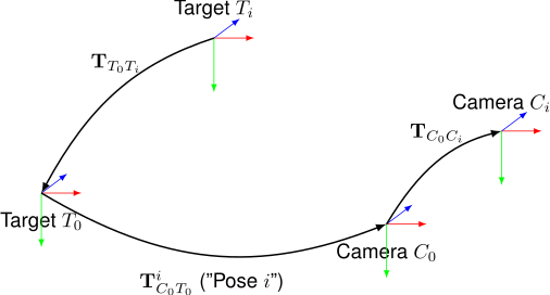
where \(\mathbf{T}_{C_0T_0}^i\) (simply called Pose \(i\)) is the transform from target 0's frame to camera \(C_0\) in the \(i\)th pose, \(\mathbf{T}_{C_0C_i}\) is the camera extrinsics transform from \(C_0\) to camera \(C_i\), and \(\mathbf{T}_{T_0T_i}\) is the transform from the reference target to target \(T_i\).
Data requirements
Accurate calibration depends on the quantity, diversity, and quality of the input data. As a rule of thumb, collect enough images so that each camera model parameter is observed over multiple poses and across the full image area.
Practical guidelines
- Coverage: ensure features span the full sensor, including corners and edges. Avoid keeping the target only near the image center.
- Pose diversity: include rotations and translations that vary pitch and yaw. Slanted views are essential to constrain focal length. Periphery coverage is important for distortion estimation.
- Focus and exposure: avoid motion blur and over/under exposure. Subpixel refinement depends on sharp, high-contrast features.
- Feature counts: prefer more observations over higher model complexity. If uncertainties are large or parameters are highly correlated, reduce model complexity or collect more data.
Network calibration
A unique feature of Calib GEOM and libCalibGeom is that multiple targets can be used to cover larger fields-of-view. ChAruCo, Kalibr, and ArUco targets/markers are the target types supported for this. Network calibration works with large numbers of cameras and/or targets. The relative transformations between targets are being optimized as part of the optimization routine. Hence, the assumption is that all targets are fixed relative to each other during the entire data acquisition.
For network calibration, a pose graph is built, which contains the cameras and the target observations as nodes. In order to yield a solution, this graph needs to be connected, which necessitates that at least some features are detected by more than one camera in at least one pose.
Covariance estimation
The advanced optimization procedures in libCalibGeom and Calib GEOM allow for estimation of the entire covariance structure of calibration parameters at the found solution. This gives information not only about parameter uncertainties (the square root of diagonal covariance matrix entries), but also about dependencies between parameters. For instance, the radial lens distortion parameters are often strongly correlated, indicating that a change in one of them can be largely explained or compensated by a change in another one.
Camera models
We support a number of mathematical camera models. However, different models have individual strengths and weaknesses. In model selection, main criteria usually are: accuracy (in terms of reprojection error), uncertainty in parameters, evaluation speed and invertibility.
The following models are supported:
- OpenCV compatible 18-parameter model based on the well-known Brown-Conrady model. Ref: Brown, Duane C. (May 1966). "Decentering distortion of lenses". Photogrammetric Engineering. 32 (3): 444–462.
- OpenCV Fisheye compatible model which is based on Brandt-Kannala's model. Ref: J. Kannala, and S. Brandt, A Generic Camera Model and Calibration Method for Conventional, Wide-Angle, and Fish-Eye Lenses, PAMI 2006
- MATLAB compatible Brown-Conrady model. See reference above.
- Double Sphere camera model. Modern low-parametric model capable of accurately modeling a wide variety of lenses. Analytical inverse. Ref: Usenko, Vladyslav, Nikolaus Demmel, and Daniel Cremers. "The double sphere camera model." 2018 International Conference on 3D Vision (3DV). IEEE, 2018.
- Enhanced Unified camera model. Modern low-parametric model capable of accurately modeling a wide variety of lenses. Analytical inverse. Ref: Khomutenko, Bogdan, Gaëtan Garcia, and Philippe Martinet. "An enhanced unified camera model." IEEE Robotics and Automation Letters 1.1 (2015): 137-144.
- B-Spline Warp camera model. A high-parametric image-space B-spline model suitable for pinhole-like lenses with complex distortion. Developed by Calib.io.
- B-Spline Ray camera model. A high-parametric ray-space B-spline model suitable for wide-angle and omnidirectional lenses. Developed by Calib.io.
- Central B-Spline camera model. A high-parametric camera model capable of modeling lenses extremely accurately if enough calibration data is provided. Ref: Calib.io internal.
- FOV camera model. An older model capable of describing a large variety of lenses using very few parameters. Ref: Automatic calibration and removal of distortion from scenes of structured environments. Machine vision and applications, Vol. 13, Issue 1, 2001.
- Halcon's Division area-scan camera model. Note that Sx and Sy are fixed to 1e-6 (reasonable pixel size) as they cannot be estimated jointly with Focus. Ref: https://www.mvtec.com/doc/halcon/12/en/calibrate_cameras.html
- Thin Prism camera model. Ref: J Weng et al. "Camera Calibration with Distortion Models and Accuracy Evaluation", TPAMI, 1992.
- OCamCalib omnidirectional camera model [Experimental]. Note that this model needs manual initialization. Ref: Scaramuzza, D. (2008). Omnidirectional Vision: from Calibration to Robot Motion Estimation, ETH Zurich, PhD Thesis no. 17635. February 22, 2008.
Regarding parameter names: parameters are named according to original published articles. However, Calib GEOM often employs an aspect ratio parameter for consistency. In models which have the parameter ar, the focal lengths for \(x\) and \(y\) are given by \(f_x = \texttt{f}\) and \(f_y = \texttt{f ar}\) respectively.
Often the camera model choice is dictated by external constraints, e.g. which software platform is being used with the parameter results downstream. With Calib GEOM, advanced camera models can be used to generate lens distortion maps which are then loaded into e.g. OpenCV to correct images. Alternatively, unprojection maps can be exported and used to convert a given (distorted) pixel coordinate to the corresponding ray, enabling all camera geometry operations with very low run-time overhead. The downstream processing can then be done as if the captured image was obtained with an ideal pinhole camera.